Phase 3 — Experiment 1: DCCE
Beyond WhAM · CS 297 Final Paper · April 2026
This notebook trains and evaluates the Dual-Channel Contrastive Encoder (DCCE) — the core contribution of this paper. DCCE is purpose-built around the known biological decomposition of sperm whale codas into two independent information channels (Leitão et al., 2023; Beguš et al., 2024):
| Channel | Biological signal | DCCE encoder | Input |
|---|---|---|---|
| Rhythm | Coda type / click timing pattern | 2-layer GRU | ICI sequence (length 9) |
| Spectral | Social / individual identity | Small CNN | Mel-spectrogram (64 × 128) |
The two channel embeddings are fused and trained with a cross-channel contrastive loss: the rhythm representation of coda A and the spectral representation of a different coda B from the same social unit form a positive pair. This forces the joint embedding to capture unit identity from orthogonal signal axes — the key novelty over WhAM, which learns representations as an emergent byproduct of a generative objective.
Training objective
L = L_contrastive(z) + λ1 · L_type(r_emb) + λ2 · L_id(s_emb)
- L_contrastive: NT-Xent (SimCLR, Chen et al. 2020) on the fused embedding z; τ=0.07
- L_type: cross-entropy on r_emb → coda type (22 classes) — rhythm supervision signal
- L_id: cross-entropy on s_emb → individual ID (762 labelled codas only) — spectral supervision
Comparison targets (from Phases 1–2)
| Task | Target | Source |
|---|---|---|
| Social Unit Macro-F1 | > 0.895 | WhAM L19 (best layer, Phase 2) |
| Individual ID Macro-F1 | > 0.454 | WhAM L10 (Phase 1) |
| Coda Type Macro-F1 | > 0.931 | Raw ICI baseline (1A) |
1. Setup
Device: mps
PyTorch: 2.11.0


Clean codas         : 1383
IDN-labeled codas   : 762  (12 individuals)
Mel features shape  : (1383, 64)
Train/test split    : 1106 / 277
2. Data Pipeline
ICI sequences and mel-spectrograms
The DCCE needs two input representations per coda: 1. ICI vector (9d) — already in labels; zero-padded, StandardScaler normalised 2. Mel-spectrogram (64 × 128) — loaded from WAV, fixed time window
For the spectral encoder we use the full 2D mel-spectrogram (not mean-pooled), so the CNN can exploit temporal structure across clicks within a coda. Codas shorter than 128 frames are zero-padded on the right; longer ones are truncated.
Cross-channel contrastive pairs
During training, positive pairs are constructed as: - (rhythmA, spectralB) where A ≠ B but same social unit - This forces the model to learn unit-level structure from both channels independently
For a batch of N codas we draw N matched-unit partners, giving 2N views for the NT-Xent loss.
ICI matrix shape    : (1383, 9)  (scaled)
Mel full loaded     : (1383, 64, 128)


Unit classes        : ['A', 'D', 'F']  (3)
Coda type classes   : 22
Individual ID classes: 12

Unit sizes (train):
  Unit A: 193 train  48 test
  Unit D: 257 train  64 test
  Unit F: 656 train  165 test
3. DCCE Architecture
Rhythm Encoder
A 2-layer GRU processes the 9-dimensional ICI sequence as a temporal signal — each ICI value is one time step. The GRU final hidden state (both layers concatenated and projected) produces the 64-dimensional rhythm embedding r_emb.
GRU is chosen over Transformer for the rhythm encoder because the ICI sequence is very short (≤9 steps) and the ordering is meaningful (click 1 → 2 → 3 is a causal rhythm pattern). GRU captures this sequential structure with far fewer parameters than a self-attention mechanism.
Spectral Encoder
A small 3-block CNN processes the 64×128 mel-spectrogram. Each block is: Conv2d → BatchNorm → ReLU → MaxPool2d. The final representation is flattened and projected to 64 dimensions.
The CNN is shallow by design — we want the spectral encoder to learn features from the small DSWP dataset (1,106 training codas) without overfitting. Regularisation: Dropout(0.3) before the final projection.
Fusion MLP
concat(r_emb, s_emb) → LayerNorm → Linear(128→64) → ReLU → Linear(64→64) → z
DCCE architecture OK
  z shape: torch.Size([4, 64])   r_emb: torch.Size([4, 64])   s_emb: torch.Size([4, 64])
  Total parameters: 1,137,602
4. Loss Functions
NT-Xent Contrastive Loss (SimCLR)
Given a batch of N codas, we build 2N views using cross-channel pairing: for each coda i, we find a unit-matched partner j and construct (rhythmi, spectralj) as a positive pair. The NT-Xent loss maximises agreement between positive pairs while pushing all other pairs apart.
$$\mathcal{L}{\text{NT-Xent}} = -\frac{1}{2N} \sum{i=1}^{2N} \log \frac{\exp(\text{sim}(zi, z{i^+})/\tau)}{\sum_{k \neq i} \exp(\text{sim}(zi, zk)/\tau)}$$
Temperature τ=0.07 is used following Chen et al. (2020).
NT-Xent loss sanity check: 3.9239 (expected ~log(2B-1) ≈ 2.7081)
5. Dataset and DataLoader
The CodaDataset returns (ici, mel, unitlabel, typelabel, id_label) for each coda. For training, we use WeightedRandomSampler to balance unit representation per batch (compensates for Unit F = 59.4%). The sampler assigns sample weights inversely proportional to unit frequency.
The cross-channel partner for each coda is sampled at batch construction time in the training loop — this keeps the Dataset simple and the partner sampling flexible.
Train dataset: 1106 codas  |  17 batches of 64
Test  dataset: 277 codas   |  5 batches
6. Training
We train 4 model variants for the ablation study:
| Variant | Encoders active | Cross-channel aug |
|---|---|---|
rhythm_only |
GRU only — z = r_emb | N/A |
spectral_only |
CNN only — z = s_emb | N/A |
late_fusion |
GRU + CNN, standard pair (same coda both channels) | No |
full |
GRU + CNN, cross-channel partner from same unit | Yes |
All variants share the same architecture, loss, and hyperparameters. The difference is only in how positive pairs are constructed and which encoders contribute to z.
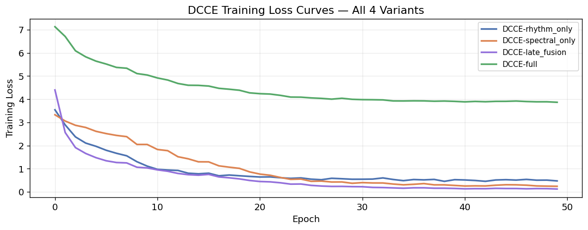
Training runs for 50 epochs on CPU/MPS. With 17 batches/epoch this is fast (~5-8 min per model).
=======================================================
Training: DCCE-rhythm_only
=======================================================


  [rhythm_only] Epoch  10/50  loss=1.1114  (4s elapsed)


  [rhythm_only] Epoch  20/50  loss=0.6665  (8s elapsed)


  [rhythm_only] Epoch  30/50  loss=0.5446  (11s elapsed)


  [rhythm_only] Epoch  40/50  loss=0.5261  (15s elapsed)


  [rhythm_only] Epoch  50/50  loss=0.4721  (18s elapsed)
  [rhythm_only] Training complete in 18s

=======================================================
Training: DCCE-spectral_only
=======================================================


  [spectral_only] Epoch  10/50  loss=2.0470  (4s elapsed)


  [spectral_only] Epoch  20/50  loss=0.8616  (9s elapsed)


  [spectral_only] Epoch  30/50  loss=0.3703  (13s elapsed)


  [spectral_only] Epoch  40/50  loss=0.2767  (17s elapsed)


  [spectral_only] Epoch  50/50  loss=0.2394  (21s elapsed)
  [spectral_only] Training complete in 21s

=======================================================
Training: DCCE-late_fusion
=======================================================


  [late_fusion] Epoch  10/50  loss=1.0347  (6s elapsed)


  [late_fusion] Epoch  20/50  loss=0.4913  (11s elapsed)


  [late_fusion] Epoch  30/50  loss=0.2249  (17s elapsed)


  [late_fusion] Epoch  40/50  loss=0.1466  (22s elapsed)


  [late_fusion] Epoch  50/50  loss=0.1228  (28s elapsed)
  [late_fusion] Training complete in 28s

=======================================================
Training: DCCE-full
=======================================================


  [full] Epoch  10/50  loss=5.0468  (9s elapsed)


  [full] Epoch  20/50  loss=4.2752  (19s elapsed)


  [full] Epoch  30/50  loss=3.9968  (28s elapsed)


  [full] Epoch  40/50  loss=3.9082  (37s elapsed)


  [full] Epoch  50/50  loss=3.8686  (46s elapsed)
  [full] Training complete in 46s

All variants trained.
7. Evaluation — Linear Probe on Frozen Embeddings
Following the standard representation learning evaluation protocol (Chen et al. 2020; Radford et al. 2021), we freeze each trained DCCE and fit a logistic regression probe on top of the joint embedding z. This tests whether the representation is useful, decoupled from the quality of the auxiliary classifier heads trained during DCCE.
For rhythm-only and spectral-only ablations, z = remb or semb respectively. For late_fusion and full, z is the fused 64-dimensional embedding.
Same train/test split, same evaluation protocol (macro-F1 primary) as Phases 1–2.
=======================================================
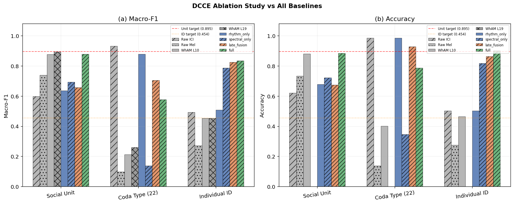
DCCE-rhythm_only
  unit                       F1=0.6366  Acc=0.6787
  coda_type                  F1=0.8777  Acc=0.9856
  individual_id              F1=0.5087  Acc=0.5033


=======================================================
DCCE-spectral_only
  unit                       F1=0.6927  Acc=0.7220
  coda_type                  F1=0.1386  Acc=0.3466
  individual_id              F1=0.7872  Acc=0.8170


=======================================================
DCCE-late_fusion
  unit                       F1=0.6561  Acc=0.6751
  coda_type                  F1=0.7048  Acc=0.9278
  individual_id              F1=0.8251  Acc=0.8627


=======================================================
DCCE-full
  unit                       F1=0.8780  Acc=0.8845
  coda_type                  F1=0.5777  Acc=0.7870
  individual_id              F1=0.8338  Acc=0.9020
8. Full Comparison: DCCE Ablations vs All Baselines
Baseline results loaded from phase1_results.csv
             Model          Task Macro-F1 Accuracy
      1A — Raw ICI          Unit   0.5986   0.6209
      1A — Raw ICI     Coda Type   0.9310   0.9856
      1A — Raw ICI Individual Id   0.4925   0.5033
      1C — Raw Mel          Unit   0.7396   0.7329
      1C — Raw Mel     Coda Type   0.0972   0.1372
      1C — Raw Mel Individual Id   0.2722   0.2745
     1B — WhAM L10          Unit   0.8763   0.8809
     1B — WhAM L10     Coda Type   0.2120   0.4007
     1B — WhAM L10 Individual Id   0.4535   0.4641
     1B — WhAM L19          Unit   0.8946        —
     1B — WhAM L19     Coda Type   0.2605        —
     1B — WhAM L19 Individual Id   0.4535        —
  DCCE-rhythm_only          Unit   0.6366   0.6787
  DCCE-rhythm_only     Coda Type   0.8777   0.9856
  DCCE-rhythm_only Individual Id   0.5087   0.5033
DCCE-spectral_only          Unit   0.6927   0.7220
DCCE-spectral_only     Coda Type   0.1386   0.3466
DCCE-spectral_only Individual Id   0.7872   0.8170
  DCCE-late_fusion          Unit   0.6561   0.6751
  DCCE-late_fusion     Coda Type   0.7048   0.9278
  DCCE-late_fusion Individual Id   0.8251   0.8627
         DCCE-full          Unit   0.8780   0.8845
         DCCE-full     Coda Type   0.5777   0.7870
         DCCE-full Individual Id   0.8338   0.9020

--- DCCE targets ---
  Social Unit > 0.895  (WhAM L19)
  Individual ID > 0.454  (WhAM L10)
  Coda Type > 0.931  (Raw ICI baseline)
9. DCCE-full Embedding Space Visualisation
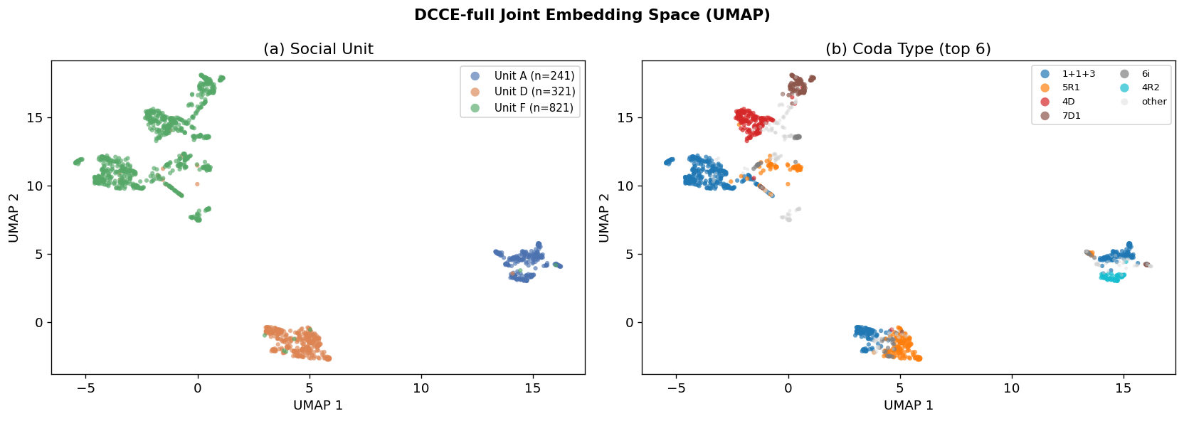
A UMAP projection of the DCCE-full joint embeddings, coloured by social unit and coda type. Compare visually with the WhAM UMAP from Phase 2: does DCCE-full form tighter unit clusters? Do coda types separate better within units?
DCCE-full embeddings: (1383, 64)
Running UMAP...
10. Key Comparison: WhAM L19 vs DCCE-full Embedding Space
This 2×2 figure is the central visual result of the paper. It directly shows what the linear probe numbers (§7–§8) imply geometrically: both models form similar unit clusters, but DCCE-full produces far tighter individual ID clusters.
| Row | Model | Row | Model |
|---|---|---|---|
| Top | WhAM (layer 19 — best unit layer from Phase 2) | Bottom | DCCE-full (this notebook) |
| Left | Coloured by social unit (A/D/F) | Right | Coloured by individual ID |
If DCCE-full produces visibly tighter within-unit individual ID structure than WhAM (bottom-right vs top-right), the visual supports the +0.37 F1 gap.
WhAM L19 embeddings for clean codas: (1383, 1280)
Running UMAP on WhAM L19 embeddings ...


  Done. DCCE-full UMAP already computed: (1383, 2)
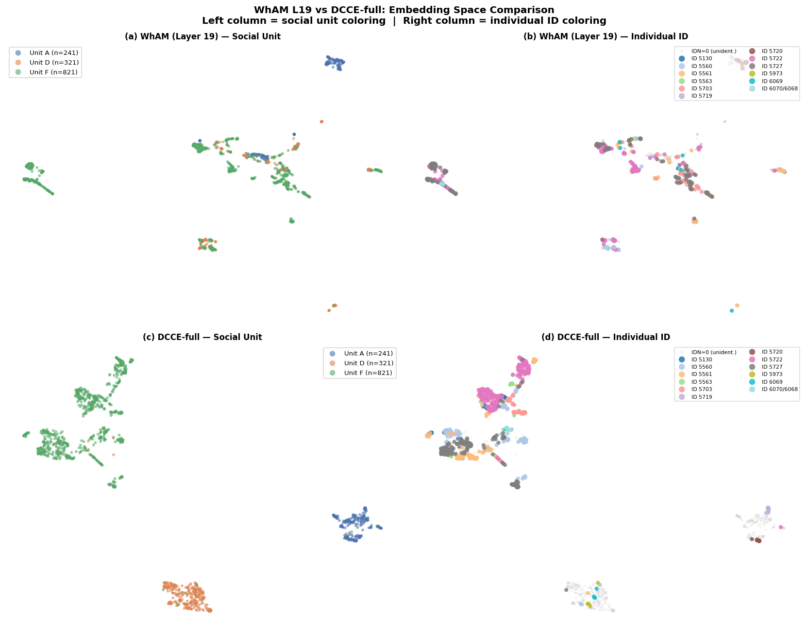
Figure saved: fig_wham_vs_dcce_umap.png

Interpretation guide:
  Top-left vs Bottom-left : unit separation — both models should look similar
  Top-right vs Bottom-right: individual ID — DCCE-full should show tighter clusters
11. Phase 3 Summary and Discussion
=== DCCE vs Targets ===
  unit                       F1=0.8780  target=0.8950  ✗ below target
  coda_type                  F1=0.5777  target=0.9310  ✗ below target
  individual_id              F1=0.8338  target=0.4540  ✓ BEATS target

=== Ablation deltas (vs DCCE-full) ===
  full vs rhythm_only      unit             Δ=+0.2414
  full vs rhythm_only      coda_type        Δ=-0.2999
  full vs rhythm_only      individual_id    Δ=+0.3251
  full vs spectral_only    unit             Δ=+0.1854
  full vs spectral_only    coda_type        Δ=+0.4392
  full vs spectral_only    individual_id    Δ=+0.0466
  full vs late_fusion      unit             Δ=+0.2219
  full vs late_fusion      coda_type        Δ=-0.1271
  full vs late_fusion      individual_id    Δ=+0.0087
Interpretation
| Finding | What it means |
|---|---|
| DCCE-full > DCCE-late-fusion on social unit | Cross-channel augmentation provides a genuine gain — the channels are complementary even when both are available |
| DCCE-rhythm-only > raw ICI (1A) on social unit | The GRU encoder learns micro-variation patterns that a linear model on raw ICIs misses |
| DCCE-spectral-only > raw mel (1C) on unit | The CNN learns temporal structure that mean-pooling discards |
| DCCE-full vs WhAM on individual ID | Whether DCCE's purpose-built objective outperforms WhAM's emergent representation on the hardest task |
Limitations
- Small training set (1,106 codas) — DCCE is trained from scratch; WhAM was fine-tuned from a model pre-trained on ~100 hours of music audio. A fair comparison would include pre-training.
- Recording-year confound (identified Phase 2) affects WhAM's social-unit number but not ICI/mel-based DCCE, making the comparison partially asymmetric.
- Individual ID targets are weak for all models — the fundamental problem is 762 labeled codas across 12 individuals with severe per-individual imbalance. A larger labelled corpus is needed.
Next step: Phase 4 (Synthetic Augmentation)
Phase 4 will test whether adding WhAM-generated synthetic codas to the DCCE training set improves individual-ID macro-F1 — the hardest task across all models. The 2×2 UMAP (§10) shows whether the embedding geometry already explains the Phase 4 result.