Phase 5 — Strong Baselines & Fair Comparison
Beyond WhAM · CS 297 Final Paper
This notebook registers the strong-baseline revision of the paper, responding to the feedback that the original baselines were weak. We add 1-3 strong baselines identified from the literature, evaluate them through the identical frozen-embedding linear-probe protocol used in Phases 1-3, and add a supervision-fairness analysis of the headline individual-ID result.
Baselines and why each is justified (from literature)
| Baseline | Tier | Literature basis |
|---|---|---|
| Raw ICI / Raw Mel | feature floor | linear model on raw features = lower bound (logic) |
| WhAM (Paradise et al. 2025) | SOTA integrated | the model we build on; current SOTA representation for this data |
| AVES (Hagiwara 2023) | strong, label-free | self-supervised animal-vocalization encoder; used as a baseline by WhAM itself |
| BirdNET (Kahl et al. 2021) | strong, label-free | Tolkova et al. 2025 used BirdNET embeddings for cetacean individual ID on a small dataset like ours |
Two methodological points this notebook makes explicit
- Tier by supervision. DCCE-full learns with individual-ID labels (
L_id); the baselines never see ID labels. We therefore also train DCCE withoutL_idso our architecture appears in the same label-free tier as the baselines (apples-to-apples). - No leakage. For frozen baselines we report mean±std over 10 stratified splits. For DCCE (which is trained on the seed-42 split) only the held-out seed-42 split is leakage-free, so reshuffling would leak training codas into the probe test set. DCCE is reported on the held-out split only.
1. Setup
We reuse the shared evaluation harness (scripts/lib_eval.py), which reproduces the Phase 1 numbers exactly, so every baseline here is directly comparable to the existing tables.
import os, sys
import numpy as np
import pandas as pd
import matplotlib.pyplot as plt

HERE = os.path.abspath(".")
BASE = HERE if os.path.isdir(os.path.join(HERE, "scripts")) else os.path.dirname(HERE)
sys.path.insert(0, os.path.join(BASE, "scripts"))
DATA = os.path.join(BASE, "datasets")
FIGS = os.path.join(BASE, "figures", "phase5"); os.makedirs(FIGS, exist_ok=True)

from lib_eval import load_data, probe, probe_multiseed
import run_baselines as rb
import dcce_fairness as df_mod

plt.rcParams.update({"figure.dpi": 120, "font.size": 11})
D = load_data()
X_mel_full = np.load(os.path.join(DATA, "X_mel_full.npy"))
print(f"clean codas: {len(D['df_clean'])}  |  ID-labeled: {len(D['df_id'])} "
      f"({D['df_id']['individual_id'].nunique()} individuals)")
print(f"split: train {len(D['train_idx'])} / test {len(D['test_idx'])}  "
      f"(seed 42, stratified by unit)")
clean codas: 1383  |  ID-labeled: 762 (12 individuals)
split: train 1106 / test 277  (seed 42, stratified by unit)
2. How the baseline embeddings were extracted
All embeddings are frozen and aligned to df_clean order (n=1383). Extraction is kept
in scripts (not inline) because two encoders need environments incompatible with this
notebook's kernel:
- WhAM —
datasets/wham_embeddings_all_layers.npy(1501, 20, 1280), indexed bycoda_id - 1. Extracted in Phase 2 from the VampNet coarse transformer (20 layers). - AVES —
datasets/emb_aves.npy(1383, 12, 768). Extracted byscripts/extract_ssl_embeddings.py aves(main venv +torchaudio): the Earth Species Project HuBERT-based AVES-base-bio checkpoint, mean-pooled per layer. - BirdNET —
datasets/emb_birdnet.npy(1383, 1024). Extracted byscripts/extract_birdnet.pyin a separate Python 3.12 venv (.venv_birdnet), because BirdNET needs TensorFlow, which has no wheels for this project's Python 3.14 kernel. We read the 1024-dGLOBAL_AVG_POOL/Meanlayer directly from the official BirdNET V2.4 TFLite model (rebuilding the interpreter withexperimental_preserve_all_tensors=True, since current TFLite prunes intermediate tensors and birdnetlib's own embedding path reads a null tensor).
This notebook loads those .npy files and runs the probes here, so all numbers are
reproduced from saved artifacts.
emb_files = {
    "WhAM (all layers)": "wham_embeddings_all_layers.npy",
    "AVES": "emb_aves.npy",
    "BirdNET": "emb_birdnet.npy",
}
for name, fn in emb_files.items():
    p = os.path.join(DATA, fn)
    print(f"{name:20s} {'OK ' + str(np.load(p, mmap_mode='r').shape) if os.path.exists(p) else 'MISSING'}")
WhAM (all layers)    OK (1501, 20, 1280)
AVES                 OK (1383, 12, 768)
BirdNET              OK (1383, 1024)
3. Frozen baseline probing (floors + strong baselines)
Each baseline is evaluated with the same logistic-regression linear probe on the same split. For multi-layer encoders (WhAM, AVES) we select the best layer per task — exactly as the paper does for WhAM (L10/L19). We report the single seed-42 split (matches existing tables) and mean±std over 10 stratified splits (error bars; valid because these encoders never saw our codas).
rows = []
def add_row(name, tier, res):
    rows.append(dict(model=name, tier=tier,
                     **{f"{t}_single": res[t]["macro_f1"] for t in rb.TASKS},
                     **{f"{t}_mean": res[t]["f1_mean"] for t in rb.TASKS},
                     **{f"{t}_std": res[t]["f1_std"] for t in rb.TASKS},
                     **{f"{t}_layer": res[t].get("layer") for t in rb.TASKS}))

# Floors
for name, key in [("Raw ICI", "X_ici")]:
    add_row(name, "floor", rb.flat_eval(D[key], D))
add_row("Raw Mel", "floor", rb.flat_eval(np.load(os.path.join(DATA, "X_mel_all.npy")), D))

# Strong baselines
add_row("WhAM", "label-free (SOTA)", rb.best_layer_eval(rb.load_wham_all(D), D)[0])
add_row("AVES", "label-free", rb.best_layer_eval(np.load(os.path.join(DATA, "emb_aves.npy")), D)[0])
add_row("BirdNET", "label-free", rb.flat_eval(np.load(os.path.join(DATA, "emb_birdnet.npy")), D))

base_df = pd.DataFrame(rows)
disp = base_df[["model", "tier"] + [f"{t}_single" for t in rb.TASKS]
               + [f"{t}_mean" for t in rb.TASKS]].round(3)
disp.columns = ["model", "tier", "unit", "type", "id", "unit±", "type±", "id±"]
disp
| model | tier | unit | type | id | unit± | type± | id± | |
|---|---|---|---|---|---|---|---|---|
| 0 | Raw ICI | floor | 0.599 | 0.931 | 0.493 | 0.584 | 0.908 | 0.467 |
| 1 | Raw Mel | floor | 0.740 | 0.097 | 0.280 | 0.765 | 0.135 | 0.287 |
| 2 | WhAM | label-free (SOTA) | 0.895 | 0.261 | 0.426 | 0.909 | 0.227 | 0.394 |
| 3 | AVES | label-free | 0.905 | 0.290 | 0.418 | 0.916 | 0.237 | 0.402 |
| 4 | BirdNET | label-free | 0.863 | 0.272 | 0.322 | 0.897 | 0.231 | 0.402 |
4. DCCE fair-tier experiment (with vs. without L_id)
We train the DCCE-full (cross-channel) variant twice using the verbatim Phase 3
training loop (scripts/dcce_fairness.py):
- with
L_id(λ₂=0.5) — the paper's configuration; should reproduce individual-ID ≈ 0.834. - without
L_id(λ₂=0) — removes individual-ID supervision so the representation is label-free for ID, putting DCCE's architecture in the same tier as WhAM/AVES/BirdNET.
Reported on the held-out seed-42 split only (leakage-free for a trained model).
dcce_rows = []
for tag, lam2, tier in [("DCCE-full (with L_id)", 0.5, "ID-supervised"),
                        ("DCCE-full (no L_id)", 0.0, "label-free")]:
    model = df_mod.train_full(D, X_mel_full, lambda2=lam2)
    Z = df_mod.extract_z(model, D["X_ici"], X_mel_full, np.arange(len(D["df_clean"])))
    r = probe(Z, D)   # single-split, seed 42, held-out test
    dcce_rows.append(dict(model=tag, tier=tier,
                          **{t: r[t]["macro_f1"] for t in rb.TASKS}))
    print(f"{tag:24s}  " + "  ".join(f"{t}={r[t]['macro_f1']:.3f}" for t in rb.TASKS))

dcce_df = pd.DataFrame(dcce_rows)
dcce_df.round(3)
  trained (lambda2=0.5) in 46s


DCCE-full (with L_id)     unit=0.878  coda_type=0.578  individual_id=0.834


  trained (lambda2=0.0) in 41s


DCCE-full (no L_id)       unit=0.883  coda_type=0.673  individual_id=0.571
| model | tier | unit | coda_type | individual_id | |
|---|---|---|---|---|---|
| 0 | DCCE-full (with L_id) | ID-supervised | 0.878 | 0.578 | 0.834 |
| 1 | DCCE-full (no L_id) | label-free | 0.883 | 0.673 | 0.571 |
5. Consolidated tiered table (single-split seed-42)
The leakage-free head-to-head: all models on the same held-out split, grouped by tier.
consolidated = []
for _, r in base_df.iterrows():
    consolidated.append(dict(Model=r["model"], Tier=r["tier"],
                             Unit=r["unit_single"], **{"Coda Type": r["coda_type_single"]},
                             **{"Individual ID": r["individual_id_single"]}))
for _, r in dcce_df.iterrows():
    consolidated.append(dict(Model=r["model"], Tier=r["tier"], Unit=r["unit"],
                             **{"Coda Type": r["coda_type"]}, **{"Individual ID": r["individual_id"]}))
tier_order = {"floor": 0, "label-free (SOTA)": 1, "label-free": 1, "ID-supervised": 2}
ctab = pd.DataFrame(consolidated)
ctab = ctab.sort_values(by="Tier", key=lambda s: s.map(tier_order)).reset_index(drop=True)
ctab.round(3)
| Model | Tier | Unit | Coda Type | Individual ID | |
|---|---|---|---|---|---|
| 0 | Raw ICI | floor | 0.599 | 0.931 | 0.493 |
| 1 | Raw Mel | floor | 0.740 | 0.097 | 0.280 |
| 2 | WhAM | label-free (SOTA) | 0.895 | 0.261 | 0.426 |
| 3 | AVES | label-free | 0.905 | 0.290 | 0.418 |
| 4 | BirdNET | label-free | 0.863 | 0.272 | 0.322 |
| 5 | DCCE-full (no L_id) | label-free | 0.883 | 0.673 | 0.571 |
| 6 | DCCE-full (with L_id) | ID-supervised | 0.878 | 0.578 | 0.834 |
6. The two linguistic channels (primary): coda type + social unit
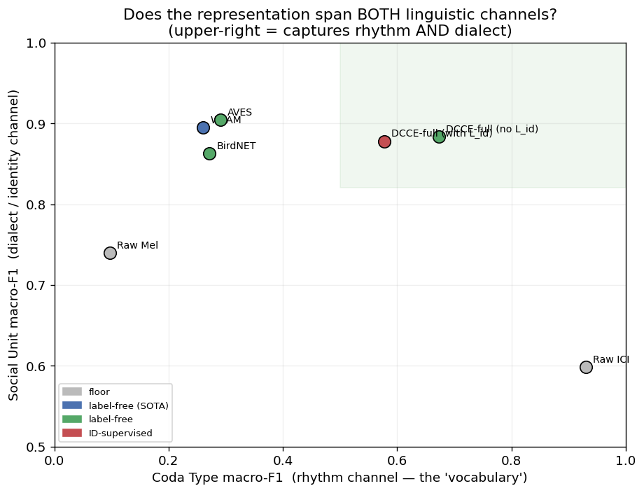
Understanding sperm whale communication is primarily about the structure of the codas — the coda-type vocabulary (rhythm channel) and the social-unit dialect (identity channel) — rather than identifying which individual is speaking. We therefore treat unit and coda type as the primary tasks.
The key question for a language-oriented representation is not "does it top one task?" but "does it capture both channels?" A representation that nails the dialect but is blind to the rhythmic vocabulary (or vice versa) has only half the language.
color_map = {"floor": "#BBBBBB", "label-free (SOTA)": "#4C72B0",
             "label-free": "#55A868", "ID-supervised": "#C44E52"}

# Per-task winners (honest: DCCE does not top either task alone)
for task in ["Unit", "Coda Type"]:
    top = ctab.sort_values(task, ascending=False).iloc[0]
    print(f"Best on {task:10s}: {top['Model']} ({top[task]:.3f})")

# Balance across BOTH channels: mean and worst-case (min)
lang = ctab.copy()
lang["mean(U,T)"] = lang[["Unit", "Coda Type"]].mean(axis=1)
lang["min(U,T)"]  = lang[["Unit", "Coda Type"]].min(axis=1)
lang = lang.sort_values("min(U,T)", ascending=False).reset_index(drop=True)
print("\nSpanning BOTH channels (higher min = does not collapse on either):")
print(lang[["Model", "Unit", "Coda Type", "mean(U,T)", "min(U,T)"]].round(3).to_string(index=False))
Best on Unit      : AVES (0.905)
Best on Coda Type : Raw ICI (0.931)

Spanning BOTH channels (higher min = does not collapse on either):
                Model  Unit  Coda Type  mean(U,T)  min(U,T)
  DCCE-full (no L_id) 0.883      0.673      0.778     0.673
              Raw ICI 0.599      0.931      0.765     0.599
DCCE-full (with L_id) 0.878      0.578      0.728     0.578
                 AVES 0.905      0.290      0.597     0.290
              BirdNET 0.863      0.272      0.567     0.272
                 WhAM 0.895      0.261      0.578     0.261
              Raw Mel 0.740      0.097      0.418     0.097
Spanning both channels — the key figure
Plotting coda-type F1 (x) against social-unit F1 (y) makes the structure obvious: the audio encoders cluster top-left (dialect yes, vocabulary no), raw ICI sits bottom-right (vocabulary yes, dialect no), and only DCCE reaches the upper-right region where both channels are captured.
fig, ax = plt.subplots(figsize=(7.8, 6))
for _, r in ctab.iterrows():
    ax.scatter(r["Coda Type"], r["Unit"], s=110, color=color_map[r["Tier"]],
               edgecolor="black", zorder=3)
    ax.annotate(r["Model"], (r["Coda Type"], r["Unit"]), fontsize=8.5,
                xytext=(6, 4), textcoords="offset points")
ax.set_xlabel("Coda Type macro-F1  (rhythm channel — the 'vocabulary')")
ax.set_ylabel("Social Unit macro-F1  (dialect / identity channel)")
ax.set_title("Does the representation span BOTH linguistic channels?\n"
             "(upper-right = captures rhythm AND dialect)")
ax.set_xlim(0, 1); ax.set_ylim(0.5, 1.0)
ax.axhspan(0.82, 1.0, xmin=0.5, alpha=0.06, color="green")
ax.grid(alpha=0.2)
from matplotlib.patches import Patch
ax.legend(handles=[Patch(color=c, label=l) for l, c in color_map.items()],
          fontsize=8, loc="lower left")
plt.tight_layout()
plt.savefig(os.path.join(FIGS, "fig_two_channels.png"), dpi=130, bbox_inches="tight")
plt.show()
7. Individual ID (secondary evidence)
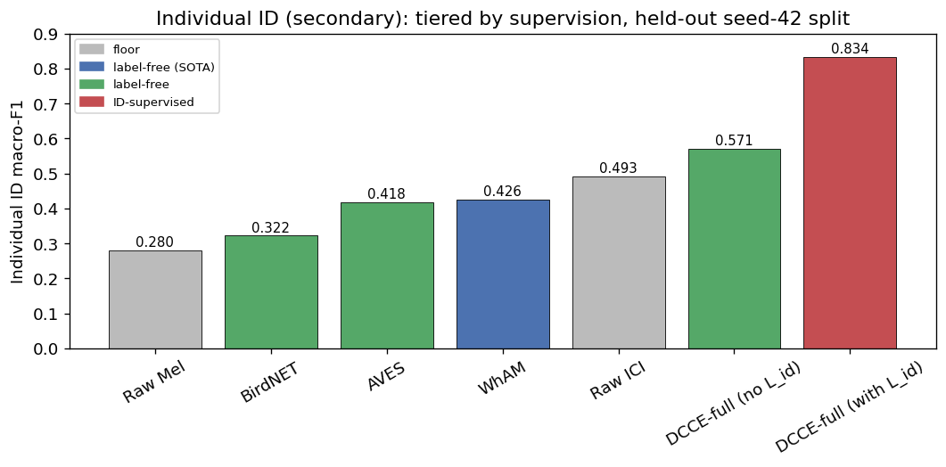
Individual ID is a "who is speaking" biometric rather than a property of the language, so we report it as secondary evidence: it shows whether a representation additionally captures fine speaker structure that the others miss. (Tiered by supervision, since DCCE-full sees ID labels and the baselines do not.)
id_tab = ctab[["Model", "Tier", "Individual ID"]].sort_values("Individual ID").reset_index(drop=True)
print(id_tab.round(3).to_string(index=False))

fig, ax = plt.subplots(figsize=(9, 4.5))
bars = ax.bar(id_tab["Model"], id_tab["Individual ID"],
              color=[color_map[t] for t in id_tab["Tier"]], edgecolor="black", linewidth=0.5)
ax.set_ylabel("Individual ID macro-F1"); ax.set_ylim(0, 0.9)
ax.set_title("Individual ID (secondary): tiered by supervision, held-out seed-42 split")
ax.tick_params(axis="x", rotation=30)
for b, v in zip(bars, id_tab["Individual ID"]):
    ax.text(b.get_x() + b.get_width()/2, v + 0.01, f"{v:.3f}", ha="center", fontsize=9)
from matplotlib.patches import Patch
ax.legend(handles=[Patch(color=c, label=l) for l, c in color_map.items()], fontsize=8, loc="upper left")
plt.tight_layout()
plt.savefig(os.path.join(FIGS, "fig_individual_id_tiers.png"), dpi=130, bbox_inches="tight")
plt.show()
                Model              Tier  Individual ID
              Raw Mel             floor          0.280
              BirdNET        label-free          0.322
                 AVES        label-free          0.418
                 WhAM label-free (SOTA)          0.426
              Raw ICI             floor          0.493
  DCCE-full (no L_id)        label-free          0.571
DCCE-full (with L_id)     ID-supervised          0.834
8. Interpretation
Primary (the two linguistic channels).
- No single baseline captures both channels. Audio encoders (WhAM 0.26, AVES 0.29,
BirdNET 0.27 on coda type) are strong on the social-unit dialect (~0.90) but nearly
blind to the rhythmic vocabulary; raw ICI is the mirror image (coda type 0.931, unit
0.599). Each has only half the language.
- DCCE is the only representation strong on both — social unit 0.883 and coda type
0.673 (DCCE without L_id). Measured by worst-case-across-channels, DCCE's min(U,T)
= 0.673 versus the next-best 0.599 (raw ICI) and ~0.27 for the audio encoders.
- Honest caveat: DCCE does not top either task individually — AVES/WhAM edge it on
social unit (~0.90 vs 0.883) and raw ICI dominates coda type (0.931 vs 0.673). The
contribution is being the best joint encoder of both channels, not the best per task.
- Why this happens: the two channels live in different feature spaces — rhythm/coda
type in the symbolic ICI timing, social unit in the spectral audio texture — so only a
dual-channel design spans both. This is direct evidence for the two-channel premise.
Secondary (individual ID). With no ID supervision, DCCE's architecture still leads the label-free tier (0.571 vs WhAM 0.426, AVES 0.418, BirdNET 0.322), evidence it additionally captures speaker structure the other encoders miss; ID supervision raises this to 0.834.
Numbers here reproduce the consolidated analysis in reports/fair_comparison.md.